Hasiera »   Gai librean »   Errorea "h"-z ala "h"-rik gabe?

Error with or without h?

• Zabaldu:
• Twitter
• Facebook
• Emaila

In some languages it has sound, in others it does not. In Basque, although it is there when it is cold, it does feel, but it is not heard. If the wind has it in Basque and, although its worm is heard, there is no "h". The mistake is not in Basque, but it can be carried with mathematics. And the "H" also has its silent function in mathematics.

Although in some languages it is not pronounced, "h" performs its function in any language, since a word is not the same without "h" or "h". It is not the same to catch something (turning it into a thread) as to act on something; that something is “concave” (strings) or that someone is “contrary”. Similarly, the error is also different without h or h. Sometimes the word with h and without h can be connected even if they are of different meaning. It is about listening to hear in English and if you lose the “h” becomes ear, it seems that you lose the “h” to not disturb the ear. The error that is calculated in h and without h are also connected, since both are measures of something that has not been done correctly. Also important is the place that occupies the letter "H" in the word: the function can be concave or convex; the child, on the other hand, is Chinese or proja. The commutative property of multiplication makes mathematics indifferent to the position of “h” in error, as it depends on whether or not “h” exists.

Different error estimation

If a differential equation cannot be solved analytically, it can be solved by numerical methods. The analytical result is accurate, while the result obtained by the numerical method is approximate and is built step by step. The error in releasing a differential equation by numerical method is the difference between the exact and approximate result. A concept that theoretically has no more difficulties than a subtraction, when it must be calculated in practice becomes a complex concept. But what is the problem? We do not know the exact results of many differential equations. Therefore, by ignoring the exact result, it is impossible to calculate the error we are making when using the numerical method. Although we do not know the error, we know that the approximate result obtained using high order numerical methods is more accurate than that obtained with lower order numerical methods. However, whenever a step is taken by the numerical method, a measure is usually used that tells us whether the result obtained in that step is valid or not. What is this measure if we have said that the error cannot be calculated without knowing the concrete result?

The measure used is the estimation of the error. A very useful error estimation is calculated as the difference of results obtained using numerical methods of successive order, based on the elimination of the result obtained by using a numerical method of order ( n+1), which is known as local extrapolation. When we use it, at each step we demand that the difference between the results obtained by two consecutive methods be less than a previously established tolerance. If the condition is met, the result given by the order method ( n+1) is accepted, otherwise it will be necessary to repeat the step operations and test it with another step less than that used previously. If we wanted to use local extrapolation of any of the measurements to be carried out in a laboratory, two measurements of the amount to be measured using two different precision devices would be made. Since the precisions of these devices must be consecutive, when a higher precision device is available, the second one will be the one with greater precision among the devices with less precision than the first. In this way, we would ensure that we are using devices with successive precision. The measure should be repeated until the difference between the two measures is less than a given value and, if the condition is met, the result of the most accurate device will be accepted. As can be seen in the laboratory example, ignorance of the actual result is paid by doubling the number of calculations.

Local extrapolation is therefore a safe but expensive resource at the same time. Since its potential is based on comparing the results obtained with two different methods, it will always mean an increase in the number of calculations. Taking advantage of the certainty of local extrapolation and accepting the increase in the number of calculations, many of the creators or parents of numerical methods have focused on the design of methods that could make this number of calculations not double, that is, they have aimed to give birth to two methods of successive order with the smallest possible differences. In this sense, by using a different set of constants in a single operation, the methods that perform a method of order n or ( n+1) are very useful, since they manage to optimize the difference between two methods of successive order. Example of this are the Runge-Kutta methods introduced. In them, it is sufficient that, in addition to the operations performed to obtain the result by the order method ( n+1), a single operation is carried out to obtain the result provided by the order method n. They therefore offer an economical option to obtain results from different orders. There is only another cheaper option than getting both at the price of one. But that is impossible, because different methods must be differentiated into something.

Estimation with h without h

In numerical methods, the letter "h" is used to indicate the step size. Knowing the exact result of the initial point, a step of size "h" is given in which the approximate result of the differential equation is calculated by the operations that the numerical method requires us. Using the approximate result obtained at the new point the process is repeated. To measure the error in each step, estimates of two types are usually used: one, called estimation per step unit, pure difference between the results obtained by consecutive methods (without h); and another, called estimation per step, which is obtained by multiplying the difference between the results by the size of the step (“h”). Of course, the estimate with h and without h are not the same. Suppose we have an estimate of the error per step unit. Since the sizes of the steps usually used are smaller than the unit, the estimate obtained by multiplying this estimate by “h” is less than the one we have previously. Consequently, it can happen that an estimate not inferior to the tolerance established without multiplying by “h”, after multiplying by “h”, below the tolerance, that is, that the smallness of the step has helped to pass the barrier. In addition, the estimation multiplied by “h” gives a special advantage to small steps, since by multiplying the estimate by a lower “h”, the new estimate will be lower. In other words, the estimation per step unit (without h) places the barrier at the same height. The estimate obtained by multiplying by “H” lowers the barrier to all steps. The smallest steps are the small ones.

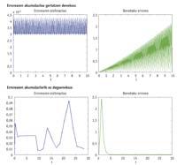
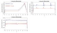
Sometimes the drop in the barrier will not be affected, as there will be estimates that would pass the initial height of the barrier without help. But there will be leaps that cannot exceed the initial height of the barrier and that will be affected by the descent of the barrier. Consequently, the step that should be repeated using another estimate will be considered valid. Repeating a step involves testing with smaller steps, and if the steps are small, more is needed. Therefore, when we use the estimates in which we are lowering the barrier, fewer steps will be taken and therefore greater than those that do not fall. The coin, however, has another aspect, since it may happen that the descent of the barrier does not have the desired result. This can negatively influence the final error and drastically reduce the quality of the approximate result we get. In general, the estimate that is calculated without h will lead to the need to take smaller steps, but the accumulation of real error will also be lower.

Estimation error in h or without h

Differential equations can be rigid or not rigid. The practical definition of the rigid differential equation is that of an equation that must take many steps to an algorithm. Although the word "much" does not indicate specific numbers, 100 steps are not many and 3,000 are many. When the problem is rigid, it is preferred to use an estimation without “h”, since with the estimation with “h” a much better result will be obtained than that obtained with the estimation without “h”. Although the problem is not rigid, the result obtained with an estimation without h will be, in most cases, better than that obtained with h, but the result --difference between both - will not be so spectacular, that is, the additional work that involves the use of an estimation without h in non-rigid differential equations will not generate much brightness in the solution.

In languages it is common for a word to lose or gain the "h" according to the time. Examples of this are the construction of walls sometimes with or without h, or the healing of patients in hospitals with or without h. However, the function or meaning of the words that have stuck or removed the “h” by the time has remained the same. The subject of errors with h and without h in mathematics does not depend on the time: there has always been coexistence between both, and both are necessary because the function of one and the other has never been the same. As we consult in the dictionary whether a word has an “h” or not, to decide whether or not to use an “h” in the estimation of the error we will have to “consult” the problem to be released, since the key to the success we will obtain in the result will be that the estimation of the error has an “h” or not.