
Mathematica (III)
3. Conditioned ends of a function
• Statement
Many times, when calculating the ends of a function, they give us the conditions that must meet those ends. That is, we will only have to accept some results. In the following example, we will see how the conditional ends of a function can be calculated using Mathematica.
• Resolution steps
We will first calculate the normal ends of the function and then compare them to the conditioned ends. We will calculate the conditioned ends using the Lagrange multiplier method.
• Commands to use
D: calculates the derivative of a function with respect to the given variable.
Solve: is the order of solving equations.
Union: makes list collection by removing repeated elements.
/: applies the rule or set of rules to the right to the left expression.
Plot3D: makes a three-dimensional image of a function.
ViewPoint: displays the three-dimensional image from a specific point of view.
AspecRatio: represents the ratio of the axis of the graph.
DisplayFunction: lets you view the chart or not.
<unk> Range: allows you to limit function values in the chart.
Axes: characteristic of representing or not the axes of the graphics.
Boxed: represents the box in three-dimensional images.
RGBCodor: used to select the color of the image of a chart.
Point Size: indicates the size of the point in the image.
Point: Adapts the bands of two or three elements to a plane or point of space.
Show: shows graphic components.
ParametricPlot3D: performs a three-dimensional graph from parametric equations. It is used to represent surfaces that cannot be expressed as functions.
Box Ratios: allows to express the proportions between the axes of the three-dimensional graphics.
Contour Plot: represents the level curves of a three-dimensional image.
ParametricPlot: two-dimensional graph from parametric equations. It is used to represent curves that cannot be represented as functions.
<unk> Style: allows you to define some features of the image.
Graphics: converts the data given to it into a representative element.
Polygon: binds the points awarded by a polygon.
• Resolution by Mathematica
g[x_, y_]:= y3 + x2 and + 2x2 + 2y2 - 4y – 8
Common ends:
d1[x_,y_]:=D[g[x,y],x]d2[x_,y_]:=D[g[x,y],y]
punegon=Solve[{d1[x,y]==0.d2[x,y]==0},{x,y}]punegon=Union[punegon]
{{X B 0, and Rule -2}, {x Rule 0, and Rule -2}, {x B 0, and
B 2},{x B 0, and
B/3}{{x B 0, and -2}, {x 0, and B/3}}
d11[x_,y_]:=D[g[x,y],{x,2}]d22[x_,y_]:=D[g[x,y],{y,2}]d12[x_,y_]:=D[g[x,y],x,y]
h1[x_y_]:=d11[x,y]h2[x_y_]:=d11[x,y]d22[x,y]-d12[x,y]2
hess={1,h1[x,y],h2[x,y]}
hess / punk
{1, 4 + 2 and, -4 x2 + (4 + 2y) (4 + 6y)}{{1,
0, 0}, {1, 16/3, 128/3}
In the first point (0,-2), this method does not tell us what happens because there are themes in the series that are zero. Therefore, we cannot decide the nature of this point. In the second point (0.2/3), on the other hand, the function has a relative minimum since all the issues of the succession of barriers are positive.
p0=Plot3D[g[x,y], {x,-1,1}, {y,-3,1}, ViewPoint} {1,0.5,0.25}, <unk> Ratio False Automatic, DisplayFunction Identity, <unk> Range> All, Axes False, Bose False]
-Surface Graphics-
mut=Graphics3D[{{RGBCodor[0.5.0.0.5], Point[0.03], Point[{0,-2.g[0,-2]}], {RGBCodor[1.0.0], Point[0.03], Point[{0.2/3.g[0]+0.1}]
-Graphics3D-
Show[p0, mut, DisplayFunction:>$DisplayFunction]
-Graphics3D-
Conditioned ends:
Condition x2+y2=1
F[x_,y_]:=g[x,y]+l(x2+y2-1)
d1F[x_,y_]:=D[x,y],x]d2F[x_,y_]:=D[F[x,y],y]d11F[x_,y_]:=D[F[x,y],{x,2}]d22F[x_,y,12_]:
pungel=Solve[{d1F[x,y]==0.d2F[x,y]==0.x2+y2==1}, {x,y, l}]
{{l Territory -(5/2), x Rule 0, and Rule
-1},{l -(3/2), x Rule 0, and Rule 1}
h1F[x_,y_]:=d11F[x,y]h2F[x_,y_]:=d11F[x,y]d22F[x,y]-d12F[x,y]2
hessF={1,h1F[x,y],h2F[x,y]}
{1, 4 + 2y + 2l, -4 x2 + (4 + 2y + 2l) (4 + 6y + 2l)}
hessF / pungel
{1,-3,21}, {1,3,21}
Therefore, in the first point, (0,-1), has a minimum and in the second, (0,1), the maximum, according to the signs of the themes of the succession of fences.
zi=ParametricPlot3D[{Cos[t], Sin[t], z}, {t,0,2>}, {z,-10,0}, Box Ratios Regla Automatic, DisplayFunction Identity]
-Graphics3D-
p1=Plot3D[g[x,y],{x,-1,1},{y,-3,1}, Box Ratios Rule Automatic, DisplayFunction Rule Identity]
Show[p1, zi, DisplayFunction:>$DisplayFunction,ViewPoint
B {1,0.5,8}]
-Graphics3D-
ps1=Graphics3D[{{RGBCodor[1,0,0], Point[0.025], Point[{0,1,-9}]}], {RGBCodor[0,0,1], Point[0.025], Point[{0,-1,-3}]]
-Graphics3D-
mb1=ParametricPlot3D[{Cos[t], Sin[t], -3Sin[t]-6}, {t,0,2{}, ViewPoint
{1,.0.5,8},DisplayFunction> Identity]
-Graphics3D-
Show[mb1, ps1, DisplayFunction:>$DisplayFunction]
-Graphics3D-
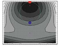
kp2=ConchannPlot[g[x,y], {x,-2.5,2.5}, {y,-3,1},
<unk> Ratio> Automatic,DisplayFunction Rule
Identity]
-Contour Graphics-
mb2=ParametricPlot[{Cos[t], Sin[t]}, {t,0.2}, <unk>
Style> RGBCcolor[0,1,0],
<unk> Ratio Set
Automatic,DisplayFunction Identity]
-Graphics-
ps2=Graphics[{{RGBCodor[1,0,0], Point[{0.06], Point[{0,1}]}, {RGBCodor[0,0,1], Point Size[0.06], Point[{0,-1}]]
-Graphics-
mut2=Graphics[{{RGBCodor[0.5.0.5],Polygon[{-0.025,-2.025},{-0.025,-1.975},{0.025,-1.975},{0.025,-2.025},{-0.025,{-0.025},{-0.025},{-0.025,}
-Graphics-
Show[kp2, mb2, mut2, ps2, DisplayFunction:>$DisplayFunction]
-Graphics-
• Comments
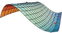
First, we have calculated the normal extremes using the traditional method. That is, we calculate the first partial derivatives using order D and solve the equation system that is generated by matching zero through Solve. The Union order has been used to remove repeated system solutions. Finally, with the second partial derivatives we have completed the succession of barriers and have determined the ends according to the succession corresponding to each point. These ends can be distinguished in the image made with the Plot3D, Graphics3D and Show commands.
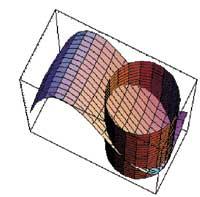
In the second part the Lagrange method has been used to calculate the conditioned ends. For this we have validated as before orders D and Solve. The three-dimensional images of function and condition were then made using Plot3D and ParametricPlot3D. Below is the intersection curve between function and condition and the points found with the Graphics3D, ParametricPlot3D, Point and Show commands.
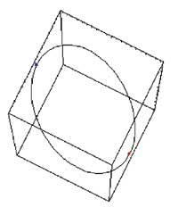
Finally, a superior projection of function and condition (Contour Plot) in which the normal ends (Polygon, square) and conditioned (Point, circle) have been placed.
Zu idazle
Zientzia aldizkaria