

Mathematica (and IV)
4º Volume delimited by the two surfaces
- Statement
We now calculate the volume delimiting both surfaces in space. For this we will use a double integral. To define the boundaries of integrals, we will represent surface projections from different points of view.
- Resolution steps
We will first calculate the normal ends of the function and then compare them to the conditioned ends. We will calculate the conditioned ends using the Lagrange multiplier method.
- Instructions to use
- ParametricPlot3D: performs a three-dimensional graph from parametric equations. It is used to represent surfaces that cannot be expressed as functions.
- ViewPoint: displays the three-dimensional image from a specific point of view.
- DisplayFunction: lets you view the chart or keep it hidden.
- Show: will show the graphic components.
- Graphics: will convert the data given to a representative element.
- Circle: with center and radius represents the circumference.
- Disk: with center and radius represents the circle.
- Rectangle: represents the rectangle with the lower left and upper right vertices.
- RGBCodor: color of a graphic image.
- Axes: characteristic of representing or not the axes of the graphics.
- AspecRatio: characteristic of representing the proportion between the axis of the graph.
- ViewPoint: displays the three-dimensional image from a specific point of view.
- Integrate: calculates the integral. Using two variables, calculate the double integral.
- Simplify: simplifies an algebraic expression.
%, refers to the previous result.
- Resolution by Mathematica
Cartesian equations:
sphere x2 + y2 + z2 = Cylinder 4: x2 + y2 - 2y = 0Parametric equations:
Dial: | x = 2cos[t] cos[v], | cylinder: | x = 2sin[t] cops[t], |
| and = 2sin[t] cos[v], | and = 2sen[t]2, | ||
| z = 2sen[v], | z = z |
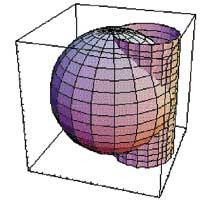
Three-dimensional image:
e = ParametricPlot3D[{2cos[t]cos[v], 2sin[t]cos[v], 2sin[v]}, {t,0,2ler}, {v,-cer/2,ler/2}, View>{3,1,1.5}, DisplayFunction <Identity]
-Graphics3D-
z = ParametricPlot3D[ {2sin[t]cos[t],2sin[t]2,z}, {t,0,2{}, {z,-2,2}, ViewPoint Rule {3,1,1.5}, DisplayFunction> Identity]
-Graphics3D-
Show[e, z, DisplayFunction: $DisplayFunction]
-Graphics3D-
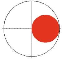
Plant projection:
pc=Graphics[{Circle[{0,0},2], {RGBCoso[1,0,0], Disk[{1,0},1]}, Axes> True, <unk> Ratio Automatic]
-Graphics3D-
Show[xliff-newline]
-Graphics3D-
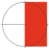
Previous screening:
Abr=Graphics[{{RGBCsmell[1,0,0], Rectangle[{0,-2},{2,2}]}, Circle[{0,0},2]}, Axes- True, <unk> Ratio-Automatic]
-Graphics3D-
Show[abr]
-Graphics3D-
Projection from the right:
epr=Graphics[{{RGBCsmell[1,0,0], Rectangle[{-1,-2},{1,2}]}, Circle[{0,0},2]}, Axes> True, <unk> Ratio Rule Automatic]
-Graphics3D-
Show[epr, Axes> True]
-Graphics3D-
Double integral:
Limits of integrals in Cartesian coordinates:
and Prudencio [0, 2],x Suitable [-] (2 and - y2), » (2 and - y2)]integrated: z = » (4 - x2 - y2).Limits of integrals in cylindrical coordinates:
integrating
z = r * (4 - r2)Note: with these limits we will only calculate the upper half of the volume.
Integrate[r*Sqrt[4-r2],{t,0,{},{r,0,2sin[t]}]?8/3
+ 4/9 (-4 + 3ess) - 4/9 (4 + 3?)
Simplify[%]
8/9 (-4 + 3ler)
This is the upper half of the volume. Therefore, the total volume:
2 * 16/9
(-4 + 3ash)
- Comments
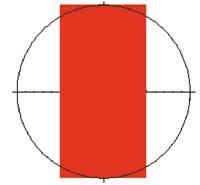
First we made a three-dimensional image to capture the idea of volume. For this we have used the traditional ParametricPlot3D and Show commands and have chosen the standard approach through the ViewPoint feature. Next, we have represented the three volume projections, top, front and right, using the Disk, Rectangle, Circle, Graphics and Show commands. In it we have also taken advantage of DisplayFunction, RGBC odor, <unk> Ratio and Axes. Finally, we calculated the double integral with the Integrate order and simplified the result using Simplify. In this way we have achieved half the volume. The total volume is obtained by multiplying the previous result (%) by two.
Zu idazle
Zientzia aldizkaria