

Differential equations in search of stability

Utility of differential equations
A mathematical model is a device that describes a system or event of life. The formulation of a mathematical model begins with the identification of the variables that influence the system, that is, they produce a change in the system. The following are reasonable hypotheses on the system, identifying the applicable empirical laws. Some of these hypotheses indicate the measure of the variation of some of the previously defined variables. The mathematical statement of these hypotheses will be an equation or a system of equations in which derivatives appear, which is the system of differential equations.
Its concrete resolution will allow us to know the behavior of the system. But, what do we talk about when we talk about model or mathematical model?
In the kinetics of chemical reactions, its evolution is interesting over time. Being the velocities derived from the time of any variable, the kinetic reaction is modelled by differential equations. An example of this is the case in which both substances generate a third. The variables are concentrations of substances, while empirical laws are the law of mass action and the law of mass conservation. The first one tells us that the product of the concentrations of the reagents is proportional to the product of the concentrations of the products, and the second, the sum of the masses of the reagents is equal to that of the products.
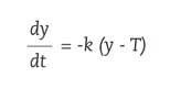
Differential equations are also used in the cooling of the bodies. For example, if we remove a cake from the oven at 150ºC and want to know its temperature at any time. If we are investigating the murder or murder of a person and want to calculate what time he died, we will use Newton's refrigeration law. This law establishes that the change in body surface temperature is proportional to the difference between body temperature and ambient temperature. Thus, if the body temperature in the instant t is y ( t ) and the temperature in the middle T, according to Newton's law, the following differential equation will be fulfilled:
Being k 0 the constant proportionality.
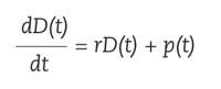
Do we want to calculate the interests that will give us a quantity of money that we enter in the bank? We must use differential equations. Suppose we introduce in the bank the amount D 0 and pay us an interest rate r. We will call D ( t ) the amount we will have within t years. The variation of the amount will be the sum of the variation by accumulation of interests and the variation of income we make in the bank, p of formula.
There is, therefore, to model in everyday life using differential equations.
Difficulties of resolution
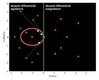
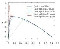
Once the differential equation is obtained, it must be resolved. Sometimes, its analytical release is not possible, and through numerical methods an approximate result is obtained. Differential equations include complex self-values which we will call l. When the real part of these autovalues is positive, the differential equation is unstable and the approximate result that we would get using a numerical method for their release does not have to resemble the real solution, since a small change has a strong impact on them. For this reason, the numerical methods are applied to stable differential equations, autobalioids of negative real part. On the other hand, the method itself also has a stability zone. And if you want to achieve a good result, self-values must be placed there. Therefore, the autovalues of stable differential equations not present in this zone are transferred to the zone of stability, multiplying the autovalues by a measured number h (0.1) that we will call step measure.
The measure of the step is fundamental to solve the equation and, of course, it cannot be any number. In terms of reliability, the resolution method must be small enough to be kept within the stability zone, and large enough to take as few steps as possible for the job. How to achieve that balance?
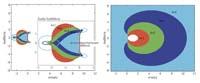
Balance of the stability area
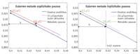
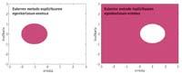
To know what steps can be taken in the numerical method, you have to look at the error. When using numerical methods, a local error is generated at each step. But there is another error that appears in length, which is the reproduction of the errors of each step, and which is formed by the powers of a number called amplification factor. To avoid the increase in error, the amplification factor must be less than the unit. The zone that meets this condition is known as the stability zone of the method. Well, the l-value should be in the stability zone after multiplying by h so that the amplification factor is less than the unit. But not only that, once the product l .h is in the stability zone, it is seen if the number h should be smaller, since any number that is less than h we have found makes it possible that after multiplying the autovalue it will be carried to the zone. Of the numbers that allow to carry the autovalue to the field, the number h that maintains the local error within a tolerance is the one chosen as the measure of the step. This step measure allows the two errors (local and longitudinal) to be controlled. The greater this number, the greater the number of steps we can take and the faster the result will be, a goal that the great stability field allows to reach.

The method itself also conditions the measurement of the stability zone. Implicit methods usually have a greater stability area than explicit ones, but they also have disadvantages: the main one is that more or less complex operations are required than in explicit methods. Therefore, when self-values are not very large, the explicit method is preferred, since the operations to be carried out will be more sustainable.
The dream would be to find maximum stability in high orders and explicit methods, but neither in this field of science is there rarity. In order to get differential equations to be easily released by numerical methods, there are numerous work done to increase the stability field. The first are the methods of Adams Bashforth and Moulton, in which the information of the last step is used as well as the information of other faster steps to build the next step. In this way, the order of the numerical method was raised, and that of order 1 has a field greater than that of explicit Euler (also of order 1). One of the most important proposals was the so-called BDF (backward differentiation formula) made by Gear around 1971, an implicit method that used information in several lighter steps. The BDF method made stability zones also important in high orders. Lately, the methods that use derivative 2 or the so-called superfuture points predominate, since they have large areas of stability, although they increase the work to be done in each step.
Many small steps or few big steps, there is the key. In this competition, the first option, with many small steps, has the advantage of reliability and the second job optimization. Unifying both options on one occasion would be excellent, as it would achieve "reliability without excessive work." The key to breaking this balance lies in methods of great stability field, which do not put such rigid limits to the measure of the step. Therefore it is possible to take steps not so reliable and great reliable steps.
Zu idazle
Zientzia aldizkaria