

Mathematica
To learn more about the story, let's say that the first version of Mathematica came out in 1988 for Apple Macintosh computers, but was quickly developed for use on other platforms: IBM PC, Silicon Graphics, Hewlett Paccard, Sun, etc… The second version was released in 1991 and has been the one used on computers until September last year, when the third version ended: Mathematica 3.0. They are basically similar. The most significant modification is the set of characters used to express mathematical expressions ( mathematical typesetting). The new mathematical symbols have a typographical and functional meaning. For example, each operation had its code or word key in previous versions. In this latest version, most operations can be expressed by both word key and mathematical writing. For example:
Power[2,10] or
210 Sqrt[28] or “w28”
At the same time, files created by Mathematica version 3.0 are Mathematica's own expressions, allowing them to be manipulated in programs like any other symbolic expression. The computing capacity is also higher in this version, with higher execution speed and lower memory in some operations. New features and tools have also been incorporated, and new ones have been improved. Also mention that it is necessary to have a computer majo enough to use this latest version comfortably, since they recommend 16 MB of Ram and 75 MB of hard disk. To conclude, indicate that all the examples to be presented will be made with Mathematica version 3.0.
Its main advantage is its ability to work with symbolic expressions. “Anything can be expressed as expressive symbolic.” That was the basic idea of those who built Mathematica. Therefore, it can be used as a numerical or symbolic calculator, it is used to visualize data and functions, it offers a high-level language to write programs, it is an ideal environment for data analysis and, above all, it is a tool capable of combining text, graphics (if desired animated) and active formulas in interactive documents. You can also handle the sound as it allows you to define sound objects.
Mathematica can perform three types of operations: numerical, symbolic, and graphic. As for numerical computing, the easiest way to use Mathematica is to use it as a calculator. However, calculators have a fixed accuracy, that is, the number of decimal figures is set beforehand, while in Mathematica the accuracy required to calculate can be indicated in the order itself. In the following example, the bold ones are the orders placed to Mathematica and in simple letter the answers given by Mathematica (the keywords In:=[number] and Out=[number] that appear above are added by the program itself to differentiate the inputs and outputs, relate each output to the corresponding input, and then make references to those inputs/outputs by a simple number).
l n[1]:=log[4pi]
Out[1]=log(4cer)
l[2]:=n[Log[4ler]] Out[2]=2.53102
ln[3]:=n[Log
4cer],10
Out[3]=2.5310247
Moreover, the set of operations is larger, about 750 functions of integral elliptical and Bessel, including factorization of hypergeometric functions and integers.
You can also apply numerical operations such as numerical integration, linear programming, etc. It also provides solutions to algebraic equations and conventional differential equations.
Among the symbolic computations he performs, the manipulation of algebraic formulas stands out. Polynomial and rational expression can be simplified, extended or factored. You can also find algebraic solutions of polynomial equations and equation systems. Unlike the second version, in the latest version it incorporates facilities to work with matrices and it is not mandatory to use tables for the definition of matrices.
It also symbolically evaluates integrals and their derivatives, handling approximations by series and calculating limits.
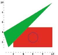
In the field of graphics, it performs two-dimensional and three-dimensional graphics, density plots and contour (top views), both from functions and from data lists. In addition, there are numerous possibilities to control the details of the chart, e.g. : focus, color, brightness…
It has a library for predefined graphics, which by means of a series of primitive orders of geometric objects (for example, polygons) displays objects graphically by a symbolic representation.
Rectangle
= Graphics[{RGBCsmell[1,0,0],
Rectangle[{2,1}, 10, 5}] rectangle
=
Graphics[{RGBCcolor[1,0,0], Angle[{2,1}, {10, 5}]>
Graphics
•Graphics•

All graphs formed by Mathematica are PostScript (PS) format so they can be transported to other applications.
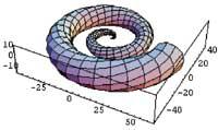
ParametricPlot3D[{uCos[u]
(4+Cos[v+u]), uSin[u] (4+Cos[v+u]), uSin[v+u]}, {u,0,4>}, {v,0,2>},
In addition, it has its own language, so you can write programs in the Mathematica language.
On the other hand, the Mathematica programming language supports different programming styles: procedural, with block structure, conditional commands and repetitive strapping; functional, with functional agents; rules-based programming, pattern matching and object-oriented programming.
The Mathematica program is structured into two large parts: the kernel and the front-end. Kernel is the kernel, the part responsible for performing the calculations, and the front-end is only the part that interacts with the user, a user-friendly interface and whose commands are sent to the kernel. If the kernel is the same on all computer platforms, we could find it with different front-end, which has been optimized for certain architectures. This front-end offers the user documents called “notebook”, i.e. priority stepped text, animated graphics and mathematical expressions (formulas, etc.) Notebooks that admits. In these notebooks you can elaborate pedagogical or other material, and the most unique feature is that, in addition to the written explanations, operations can be carried out in them.
In general, Mathematica is characterized by its communicative compatibility with many other programs. This allows you to read data in different formats (C, Fortran, TEX). By using the MathLink standard, you can exchange data and commands with other applications.
During the execution of the mathematica some static libraries are loaded. These include basic mathematical calculation functions, graphs and other common mathematical areas. However, Mathematica also has more specific libraries that are not loaded when the program starts. The loading of the packages defined for your specific needs is available to the user. For example, suppose we have defined the “factorial” and “exponential” functions in the “gurelib” library.
<unk> Package[“Calculus`gurelib`”,{”factorial”,”exponential”}]
once the order is executed, we can use the factorial and exponential operations according to the order standard given in the definition. The library that Mathematica has loaded at all times is stored in the $Packages global variable.
As it could not be otherwise, Mathematica also has its own web address, where you can find information, graphics and latest news: http://www.wolfram.com
Zu idazle
Zientzia aldizkaria